Are iBuyers manipulating the real estate market?
A preliminary analysis with Better's transaction datasetBackground
Earlier this year, iBuyers - technology companies that buy homes to sell on their platforms - were accused by some in the real estate community of so-called market manipulation. Allegations were made by influencers on social media that these companies were purchasing homes en masse to artificially drive up real estate prices in certain markets. This was echoed in anecdotes of individuals voicing their experiences of being offered unexpectedly high sums by these companies to purchase their home, inflating the cost of the home, and perhaps setting off a chain reaction of overpricing other homes in the surrounding market.
These accusations beg the question, are iBuyers manipulating the real estate market? As a mortgage lender, Better Mortgage has proprietary real estate property and transaction datasets that contain information that could help answer this question. We use this type of data across the business every day to help power a superior customer experience. The purpose of this blog post is to demonstrate the power of this data and to share some of our recent work in digging into iBuyer trends.
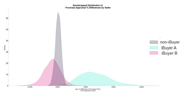
This analysis uses our customers' transaction data and property listing data to build a statistical representation of the differences between iBuyers and non-iBuyers in their transactions over the last summer. We had to accommodate for the fact that we didn't have that many iBuyer transactions in our dataset, but we were still able to interpret some striking differences in the bootstrapped distributions of the different sellers in our sample. We also used a pseudo-experimental matching technique commonly used in causal inference analysis for further rigor in comparing iBuyers to non-iBuyers in our sample.
Framing the Question
Assessing whether individual companies are "manipulating" the market is a tricky thing to define. Do we define manipulation as the impact of artificially inflating prices on the surrounding market? Going this route could pose some logistical challenges - for one, it would be difficult to determine whether an iBuyer's presence in a market causes that market to inflate or if the iBuyer's presence in a market is merely due to the fact that the market is hot! For this reason, we chose a proxy metric to define "market manipulation" in a very narrow sense of the term. Specifically, we wanted to know if iBuyers are deliberately selling overpriced homes to their clientele. Knowing whether these companies are leveraging their position in the industry to deliberately overprice their properties could provide a signal as to what their overall aims in a market are.
A key term in our approach here is deliberately. Our main challenge consists of systematically teasing out, by controlling for as many external confounding factors as possible, whether there's any evidence that these companies are overpricing their properties relative to all other comparable transactions.
Data and Approach
Data scientists and analysts at Better have access to a trove of interesting datasets that provide a window into the real estate market. Two data sources particularly relevant for this analysis are our property data and our transaction data, where, among many other features, we store information on who the entity is selling or buying a given property in each transaction. We used this seller field to partition our listing and transaction data into 4 treatment groups corresponding to whether the seller was an iBuyer, and if so, whether they were one of the top 3 iBuyers in the market:
| Seller Types |
|---|
| 1. non-iBuyer (control) |
| 2. iBuyer “A” |
| 3. iBuyer “B” |
| 4. iBuyer “C” |
At the time of writing this post, most of Summer 2021's transactions have been processed. So, a reasonable approach to constrain this investigation would be to limit our dataset to listings and transactions processed between the range 06/01/2021 - 09/01/2021. Let's take a look at some of the other key features relevant to our goal of figuring out whether iBuyers are intentionally selling overpriced homes to their customers:
| Key Feature | Description |
|---|---|
| offer_accepted_date | the date the buyer’s offer was accepted |
| median_price_of_the_market | median price at either zip or state level when there are no other listings in the zip |
| active_listings_in_the_zip | # of active listings in a zip code |
| geo (city-state) | where the home was sold |
| purchase_price | price home was sold at |
| appraised_price | price home was appraised at |
As a reminder, the key metric we're evaluating here is the relative difference of the purchase price vs appraisal price, or %_appraisal_difference, which was defined as:
((purchase_price - appraised_price )/ appraised_price ) x 100
A positive %_appraisal_difference would point to an overpriced property in a transaction while a negative would point to a good deal.
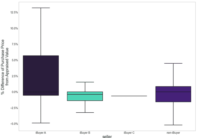
While we have enough data to assume a normal distribution of %_appraisal_difference sample means of for iBuyer A, iBuyer B, and non-iBuyers, we simply don't have enough transactions with iBuyer C in our dataset to warrant subsequent quantitative examination. With that said, let's take a look at some descriptives and boxplot visualizations for the 4 groups for our key metric of %_appraisal_difference:
| Seller | Sample Mean | 90% Confidence Intervals | Sample Size |
|---|---|---|---|
| iBuyer A | 2.59% | [-0.94%, 4.32%] | 26 |
| iBuyer B | -0.59% | [-1.31%, 4.30%] | 41 |
| iBuyer C | -0.63% | [-1.16%, 3.73%] | 8 |
| non-iBuyer | -0.01% | [-1,035%, 3.48%] | 793 |
Right off the bat we see something interesting in our sample. In our biggest group, non-iBuyers, we see a sample mean that is slightly below a 0% purchase/appraisal difference, signifying that on average in Summer 2021, Better Mortgage customers paid for homes below what they were appraised for. Put another way, we could interpret this data to mean that on average Better customers did not overpay for the homes and may have even gotten a good deal. The story appears to be quite aligned for our 41 iBuyer B transactions in the dataset, as well for our 8 iBuyer C transactions.
The story appears to be a bit different for iBuyer A, though. While not yet statistically significant, with an average %_appraisal_difference of +2.59% [0.94%, 4.32%], iBuyer A is trending towards having an average purchase price that is positive. In our sample, this means that the average iBuyer A customer may have overpaid for their home by 2.59%.
Coarsened Exact Matching
It's important to take a step back and reassess what might be going on here. A key flaw in comparing these distributions outright is that we are collapsing each group across all the different markets their transactions took place in, across all different location price tiers, time of year, and appraisal values. Simply put, there's too many confounding variables that might be driving the appearance that iBuyer A is unique from these groups.
In order to make a more apt comparison between the treatment groups, it's important to reduce these imbalances latent in the group. That's where Coarsened Exact Matching (CEM) comes in. CEM is a technique used for causal inference to reduce latent imbalances in treatment groups so as to make a more direct comparison in a certain outcome. Described another way, CEM allows multiple treatment groups to be matched to determine the existence/extent of a treatment effect. In this case, our treatment effect would be to evaluate if being a particular iBuyer company changes your distribution of %_appraisal_difference even after controlling for different market conditions and property characteristics.
Here are the features that were coarsened to match our groups:
- median_price_of_the_market
- active_listings_in_the_zip
- appraised_price
- offer_accepted_date
And here are the descriptives of the matched dataset:
| Seller | Sample Mean | 90% Confidence Intervals | Sample Size |
|---|---|---|---|
| iBuyer A | 2.79% | [0.94%, 5.00%] | 26 |
| iBuyer B | -0.63% | [-0.21%, 4.39%] | 41 |
| non-iBuyer | -0.06% | [-.33%, 4.0%] | 793 |
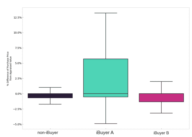
And a slightly different visualization of the same matched dataset:
It's certainly starting to be a more compelling case that iBuyer A is behaving in a categorically different way from both non-iBuyers and iBuyer B. Controlling for confounding variables and limiting the scope to zip codes where our iBuyer sellers sold properties pushed iBuyer A even further away from the pack.
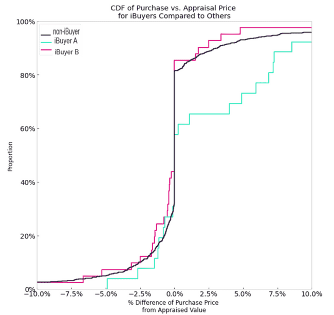
An interesting question to figure out here is what proportion of iBuyer A’s transactions with Better Mortgage’s customers exceeded a 0% appraisal difference relative to the other seller types. This type of understanding would help us determine if this visual effect is being driven by outliers.
Here are the cumulative distribution functions of %_appraisal_difference for the seller types:
This plot demonstrates how iBuyer A's sample CDF is distinct from the other groups, even after controlling for market conditions and property features. Almost 25% of iBuyer A's transactions in our dataset are greater than extreme relative purchase cost of >5% over appraisal value, compared to only ~5% or so for both iBuyer B and non-iBuyer sellers.
Quantifying the iBuyer effect
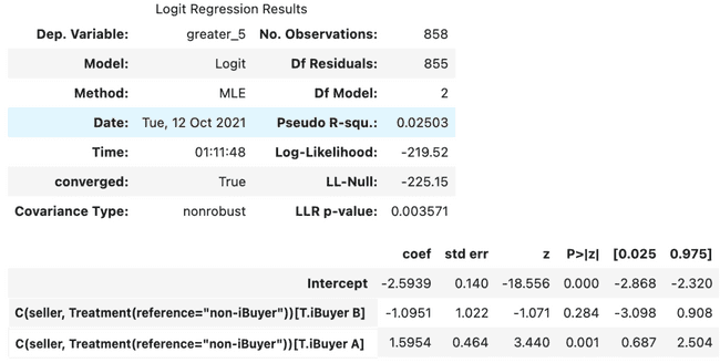
After making the observation above, it seems feasible that iBuyer A is behaving in a way that is categorically distinct from its peers - namely that it is disproportionately selling homes at a cost greater than appraisal value. But how solid is this observation from a statistical point of view? What are the odds that the effect we are seeing in our matched sample is merely due to chance? To figure this out, we could convert our initial metric %_appraisal_difference, a continuous variable, into a binary outcome that indicates whether the purchase price was at least 5% greater than the appraisal price: purchase_greater_than_5%_appraisal. Then we could model this outcome linearly as a function of the treatment group, with non-iBuyers as our reference group. When we do this, here are the results:
With a treatment logit coefficient of ~1.6, iBuyer A's iBuyer effect is the only seller type that is statistically significant (p < 0.001), and indicates that Better Mortgagecustomers who purchased their home from iBuyer A are ~5x more likely than Better Mortgage customers who purchase their home from non-iBuyer sellers to pay at least 5% more than appraisal value. The p-value here indicates that there is less than a 0.1% chance that the effect we're observing here in our sample is due to statistical randomness.
Caveated Conclusion
To reiterate, our sample of Better Mortgage customers who purchased their homes from iBuyer A, iBuyer B, and iBuyer C is likely too small to generate a representative sample of the iBuyer market nationally. That said, through leveraging causal inference methodologies and statistical modeling, we were able to identify that iBuyer A's sample in our dataset differed significantly in the purchase vs. appraisal difference from both iBuyer B transactions and non-iBuyer transactions. Specifically, iBuyer A transactions in our sample were almost 5x more likely to come in at over 5% of appraisal value and these homes' purchase prices were, on average, ~2.5% higher than appraisal value. These preliminary findings provide rationale for more companies to investigate iBuyer transactions such as these to generate a more complete picture of the practices iBuyers are employing in the real estate market.
Finally...
We are hiring! If you're interested in these types of problems, definitely let us know! We have a dynamic team of data engineers/scientists/analysts in New York City who are working on many of these types of problems on a daily basis.

Our thinking
Interning at Better
What a CS honor student learned from working at BetterTue Apr 21 2020—by Xing Tao Shi3 min read- internship
I gave the business what they asked for and they never used it
An addition to the long list of unused ML projectsMon Jun 29 2020—by Kenny Ning3 min read- data
- ML
- project management
Modeling conversion rates and saving millions of dollars using Kaplan-Meier and gamma distributions
At Better, we have spent a lot of effort modeling conversion rates using Kaplan-Meier and gamma distributions. We recently released convoys, a Python package to fit these models.Mon Jul 29 2019—by Erik Bernhardsson8 min read
