Modeling conversion rates and saving millions of dollars using Kaplan-Meier and gamma distributions

Lots of companies need to analyze conversion rates. Maybe you want to understand how many people purchased a widget out of the people that landed on your website. Or how many people upgraded to a subscription out of the people that created an account. Computing a conversion rate is often fairly straightforward and involves nothing more than dividing two numbers.

So what else is there to say about it? There is one major catch we had to deal with Better. When there is a substantial delay until the conversion event, this analysis suddenly gets vastly more complex.

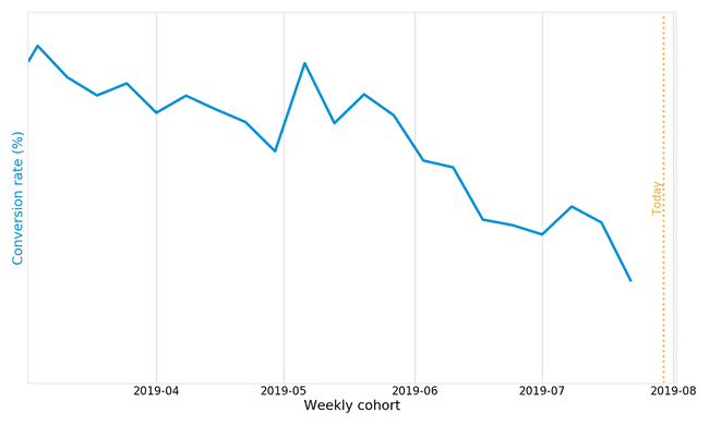
To illustrate what I am talking about, we can look at the conversion rate for borrowers coming to Better.com to get a mortgage, defined in the most simplistic way, dividing the number of converted users by the total cohort size:

This looks really bad: is the conversion rate truly going down over time? But that's not right: it only looks like it is going down because we have given the later users less time to "bake".

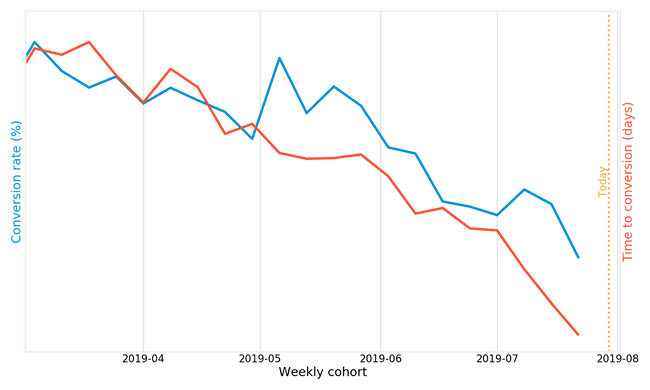
Another line shows how confusing the definition of conversion rate is. Let's look at time until conversion (right y-axis) as a function of the user cohort:

Ok, so the conversion rate is going down over time, but users are converting much faster? Clearly, this is a bogus conclusion, and yet again we are looking at it the wrong way.

(Side note, but throughout this blog post, the y scale is intentionally removed in order for us not to share important business metrics.)

The basic way: conversion at time T

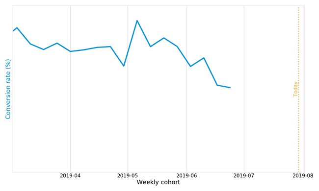
There is a few ways we can resolve this. One way is to look at conversion rate at T = 35 days, or some similar cutoff. That way we can compare and see if conversion rates are going up or down:

Sadly, this also has a pretty severe issue: we can't compute conversion rates for anything more recent than 35 days ago. Back to the drawing board!

Why does any of this matter?

It might be worth taking a step back and considering what types of issues this is causing. At Better, we spend a significant amount of money (millions of dollars) on various types of paid user acquisition. This means that we buy leads/clicks from some source, and drive traffic to our website. Some of those are high intent, some of them are low intent. Some of them can take many months to convert. This makes it challenging to answer a seemingly simple question: what's the cost of user acquisition per channel?

If we put ourselves in a position where we have to wait many months for us to measure the efficacy of an acquisition channel, that means it takes forever to iterate and improve our acquisition, and it means a lot of money thrown out the window on bad channels. So, let's consider a few better options culminating in a somewhat complex statistical model we built.

Introducing cohort models

A much better way is to look at the conversion on a cohorted basis. There is a number of different ways to do this, and I've written a whole blog post about this. I'm going to skip a lot of the intermediate steps, and jump straight to what I consider the best next point: using a Kaplan-Meier estimator. This is a technique developed over 60 years ago in the field of survival analysis.

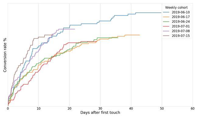
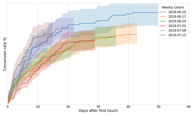
Computing a Kaplan-Meier estimator for each weekly cohort generates curves like this

The insight here is to switch from using the x-axis for the time, and instead let each cohort be its own line. These curves help us with a few things:

✅ We can compare curves for cohorts that have been "baking" for a long time and curves that just started. ✅ We don't have to throw away information by picking an arbitrary cutoff (such as "conversion at 30 days"). ✅ We can see some early behavior much quicker, by looking at the trajectory of a recent cohort.

For a wide variety of survival analysis methods in Python, I recommend the excellent lifelines package. As a side note, survival analysis is typically concerned with mortality/failure rates, so if you use any off-the-shelf survival analysis tools, your plots are going to be "upside down" from the plots in this post.

Kaplan-Meier also lets us estimate the uncertainty for each cohort, which I think is always best practice when you plot things!

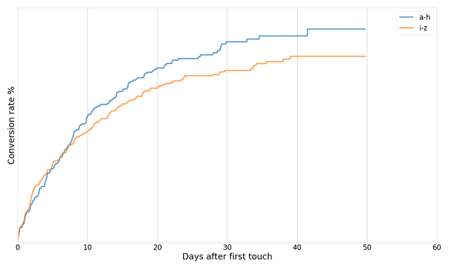
The nice thing about Kaplan-Meier is that it lets us operate on censored data. This means that for a given cohort, we're not going to have observations beyond a certain point for certain members of that cohort. Some users may not have converted yet, but may very well convert in the future.

This is most clear if we segment the users by some other property. In the case below I've arbitrarily segmented users by the first letter of their email address. These two groups contain users on a spectrum between:

• Some users that just came to our site and have essentially no time to convert
• Some users that have had plenty of time to convert

Dealing with censoring is a huge focus for survival analysis and Kaplan-Meier does that in a formalized way.

So far, so good

Ok, so this is great: we have are now checking lots of the boxes, but IMO not quite all:

✅ Can deal with censored data ✅ Can give us uncertainty estimates ❌ Can extrapolate: it would be amazing if we could look at the early shape of a cohort curve and make some statements about what it's going to converge towards.

So, let's switch to something slightly more complex: parametric survival models! Take a deep breath, I'm going to walk you through this somewhat technical topic:

Parametric survival models

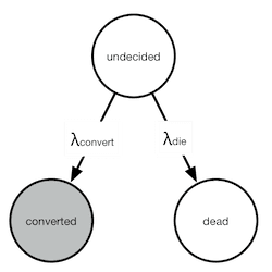
I was working on a slightly simpler cohort chart initially, and my first attempt was to fit an exponential distribution. The inspiration came from continuous-time Markov chains where you can model the conversions as a very simple transition chart:

In the chart above, we can only observe transitions to the converted state. A lack of observation does not necessarily mean no conversion, it means they are either dead, or will convert, but have not converted yet. This transition diagram actually describes a very simple differential equation that we can solve to get the closed form. I will spare you the details in this blog post, but the form of the curve that we are trying to fit is:

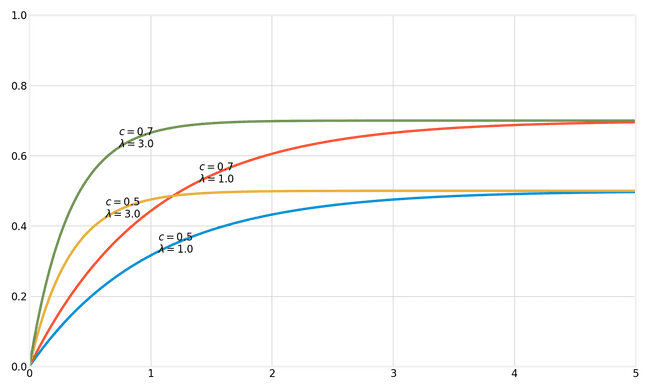
This gives us two unknown parameters for each cohort: $c$ and $\lambda$. The former explains the conversion rate that the cohort converges towards, the latter explains the speed at which it converges. See below for a few examples of hypothetical curves:

Note that the introduction of the parameter $c$ departs a bit from most of traditional survival analysis literature. Exponential distributions (as well as Weibull and gamma, which we will introduce in a second) are commonplace when you look at failure rates and other phenomena, but in all cases that I encountered so far, there is an assumption that everyone converts eventually (or rather, that everyone dies in the end). This assumption is no longer true when we consider conversions: not everyone converts in the end! That's why we have to add the $0 \leq c \leq 1$ parameter

Weibull distributions

It turns out that exponential distributions fit certain types of conversion charts well, but most of the time, the fit is poor. This excellent blog post introduced me to the world of Weibull distributions, which are often used to model time to failure or similar phenomena. The Weibull distribution adds one more parameter $p > 0$ to the exponential distribution:

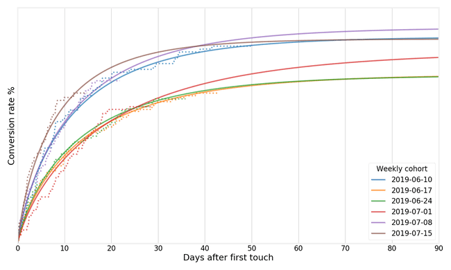
Fitting a Weibull distribution seems to work really well for a lot of cohort curves that we work with at Better. Let's fit one to the dataset we had earlier:

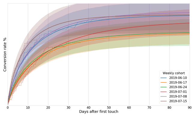
The solid lines are the models we fit, and the dotted lines the Kaplan-Meier estimates. As you can see, these lines coincide very closely. The nice thing about the extrapolated lines is that we can use them to forecast their expected final conversion rate. We can also fit uncertainty estimates to the Weibull distribution just like earlier:

The ability to extrapolate isn't just a "nice to have", but it makes it possible to make assumptions about final conversion rates much earlier, which in turn means our feedback cycle gets tighter and we can learn faster and iterate quicker. Instead of having to wait months to see how a new acquisition channel is performing, we can get an early signal very quickly, and make business decisions faster. This is extremely valuable!

Gamma and generalized gamma distributions

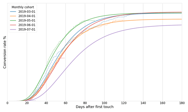
For certain types of cohort behavior, it turns out that a gamma distributions makes more sense. This distribution can be used to model a type of behavior where there is an initial time lag until conversion starts. The generalized gamma distribution combines the best of Weibull and gamma distributions into one single distribution that turns out to model almost any conversion process at Better. Here is one example:

The generalized gamma conversion model has just four parameters that we need to fit (three coming from the distribution itself, one describing the final conversion rate). Yet, it seems to be an excellent model that fits almost any conversion behavior at Better. See below for a gif where I fit a generalized gamma model to a diverse set of database queries comprising different groups, different milestones, and different time spans:

Introducing convoys

Convoys is a small Python package to help you fit these models. It implements everything shown above, as well as something which we didn't talk about so far: regression models. The point of regression models is to fit more powerful models that can predict conversion based on a set of features and learn that from historical data. We use these models for a wide range of applications at Better.

Convoys came out of a few different attempt of building the math to fit these models. The basic math is quite straightforward: fit a probability distribution times a "final conversion rate" using maximum likelihood estimation. We rely on the excellent autograd package to avoid taking derivatives ourselves (very tedious!) and scipy.optimize for the actual curve fitting. On top of that, convoys supports estimating uncertainty using emcee.

You can head over the the documentation if you want to read more about the package. Just to mention a few of the more interesting points of developing convoys:

• For a while, convoys relied on Tensorflow, but it turned out it made the code more complex and wasn't worth it.
• To fit gamma distributions, we rely a lot on the lower regularized incomplete gamma function. This function has a bug in Tensorflow where the derivative is incorrect, and it's not supported in autograd. After a lot of banging my head against the wall, I added a simple numerical approximation. Cam Davidson-Pilon (author of lifelines mentioned earlier) later ran into the exact same issue and made a small Python package that we're now using.
• In order to regularize the models, I have found it useful to put very mild priors on the variance of some of the parameters using an inverse gamma distribution. This ends up stabilizing many of the curves fit in practice, while introducing a very mild bias.
• When fitting a regression model, we have separate parameters $c_i$ and $\lambda_i$ for each feature, but shared $k$ and $p$ parameters for the generalized gamma distribution. This is a fairly mild assumption in real world cases and reduces the number of parameters by a lot.

Convoys is semi-experimental and the SDK might change very quickly in the future, but we believe it has a quite wide range of applications, so definitely check it out if you are working on similar problems!

Finally...

We are hiring! If you're interested in these types of problems, definitely let us know! We have a small but quickly growing team in of data engineers/scientists in New York City who are working on many of these types of problems on a daily basis.